Chordal Decomposition
For very large sparse semidefinite programs (SDPs) it is often helpful to analyse the sparsity structure of the PSD constraint(s). If the equality constraints impose a sparsity structure on the matrix variable, one PSD constraint on a large matrix variable can be decomposed into several smaller constraints. This results usually in a significant speedup and reduction in solve time.
The following example gives a short overview on chordal decomposition and clique merging. For more details, take a look at our paper on clique merging or watch the corresponding presentation that I gave on the topic.
Example problem
Let's consider the following SDP in standard dual form:
\[\begin{array}{ll} \text{minimize} & c^\top x \\ \text{subject to} &\displaystyle \sum_{i=1}^m A_i x_i + S = B\\ & S \in \mathbb{S}^n_+, \end{array}\]
with problem data matrices $A_1, \ldots, A_m, B \in \mathbb{S}^n$, vector variable $x \in \mathbb{R}^n$, and matrix variable $S \in \mathbb{S}^n_+$.
Let's look at the following example problem with $m=2$ and $n=9$:
A1 = [-4.0 0.0 -2.0 0.0 0.0 -1.0 0.0 0.0 0.0; 0.0 -3.0 -1.0 0.0 0.0 0.0 0.0 0.0 0.0; -2.0 -1.0 -2.0 0.0 0.0 5.0 4.0 -4.0 0.0; 0.0 0.0 0.0 -4.0 -5.0 0.0 0.0 3.0 0.0; 0.0 0.0 0.0 -5.0 4.0 0.0 0.0 2.0 0.0; -1.0 0.0 5.0 0.0 0.0 5.0 -4.0 -4.0 -5.0; 0.0 0.0 4.0 0.0 0.0 -4.0 -1.0 -1.0 -3.0; 0.0 0.0 -4.0 3.0 2.0 -4.0 -1.0 2.0 -2.0; 0.0 0.0 0.0 0.0 0.0 -5.0 -3.0 -2.0 -3.0];

A2 = [-5.0 0.0 3.0 0.0 0.0 -2.0 0.0 0.0 0.0; 0.0 -3.0 -5.0 0.0 0.0 0.0 0.0 0.0 0.0; 3.0 -5.0 3.0 0.0 0.0 5.0 -4.0 -5.0 0.0; 0.0 0.0 0.0 3.0 2.0 0.0 0.0 -2.0 0.0; 0.0 0.0 0.0 2.0 4.0 0.0 0.0 -3.0 0.0; -2.0 0.0 5.0 0.0 0.0 1.0 -5.0 -2.0 -4.0; 0.0 0.0 -4.0 0.0 0.0 -5.0 -2.0 -3.0 3.0; 0.0 0.0 -5.0 -2.0 -3.0 -2.0 -3.0 5.0 3.0; 0.0 0.0 0.0 0.0 0.0 -4.0 3.0 3.0 -4.0];

B = [-0.11477375644968069 0.0 6.739182490600791 0.0 0.0 -1.2185593245043502 0.0 0.0 0.0; 0.0 1.2827680528587497 -5.136452036888789 0.0 0.0 0.0 0.0 0.0 0.0; 6.739182490600791 -5.136452036888789 7.344770673489607 0.0 0.0 -0.2224400187044442 -10.505300166831221 -1.2627361794562273 0.0; 0.0 0.0 0.0 10.327710040060499 8.91534585379813 0.0 0.0 -6.525873789637007 0.0; 0.0 0.0 0.0 8.91534585379813 0.8370459338528677 0.0 0.0 -6.210900615408826 0.0; -1.2185593245043502 0.0 -0.2224400187044442 0.0 0.0 -3.8185953011245024 -0.994033914192722 2.8156077981712997 1.4524716674219218; 0.0 0.0 -10.505300166831221 0.0 0.0 -0.994033914192722 0.029162208619863517 -2.8123790276830745 7.663416446183705; 0.0 0.0 -1.2627361794562273 -6.525873789637007 -6.210900615408826 2.8156077981712997 -2.8123790276830745 4.71893305728242 6.322431630550857; 0.0 0.0 0.0 0.0 0.0 1.4524716674219218 7.663416446183705 6.322431630550857 0.5026094532322212];

c = [-0.21052661285686525, -1.263324575834677];
2-element Vector{Float64}:
-0.21052661285686525
-1.263324575834677Note that the data matrices $A_1,\dots, A_m, B$ all have the same sparsity pattern (common zeros in certain entries). Take a look at $A_1$:
julia> A19×9 Matrix{Float64}:
 -4.0   0.0  -2.0   0.0   0.0  -1.0   0.0   0.0   0.0
  0.0  -3.0  -1.0   0.0   0.0   0.0   0.0   0.0   0.0
 -2.0  -1.0  -2.0   0.0   0.0   5.0   4.0  -4.0   0.0
  0.0   0.0   0.0  -4.0  -5.0   0.0   0.0   3.0   0.0
  0.0   0.0   0.0  -5.0   4.0   0.0   0.0   2.0   0.0
 -1.0   0.0   5.0   0.0   0.0   5.0  -4.0  -4.0  -5.0
  0.0   0.0   4.0   0.0   0.0  -4.0  -1.0  -1.0  -3.0
  0.0   0.0  -4.0   3.0   2.0  -4.0  -1.0   2.0  -2.0
  0.0   0.0   0.0   0.0   0.0  -5.0  -3.0  -2.0  -3.0
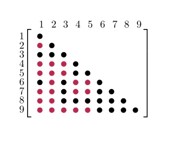
Since all the data matrices have zeros in the same places, the equality constraint of the problem tells us that our matrix variable $S$ will also have zeros in these places. The aggregated pattern matrix of $S$ is shown in the following figure, where a dot represents a nonzero entry:
Since the matrices are symmetric we only show the lower triangle. We can represent the aggregated sparsity pattern of the problem using a graph $G(V, E)$, where the vertex set $V$ is given by the column indices of the matrix and we introduce an edge $(i,j) \in E$ for every nonzero matrix element $S_{ij}$. The graph for the example problem is shown in the right figure. In order to decompose the problem, we have to find the cliques, i.e. completely connected subgraphs, of the graph $G$. These cliques represent the dense subblocks of non-zero entries in the matrix (see the colored entries in the figure). In order for the theory to work, we also have to require $G$ to be a chordal graph. For the purpose of this example, we just assume that $G$ is chordal and keep in mind that we can always make a graph chordal by adding more edges.
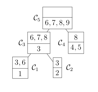
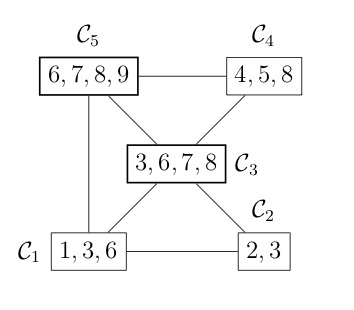
COSMO finds the cliques of the graph automatically, if a constraint of type COSMO.PsdCone or COSMO.PsdConeTriangle is present in the problem and additional equality constraints impose a structure on them. For the example problem COSMO finds the following cliques: $\mathcal{C_1}=\{1,3,6\}, \; \mathcal{C_2}=\{2,3\}, \; \mathcal{C_3}=\{3,6,7,8\}, \; \mathcal{C_4}=\{4,5,8\}$ and $\mathcal{C_5}=\{6,7,8,9\}$.
Let's denote the set of cliques $\mathcal{B}=\{\mathcal{C}_1,\ldots,\mathcal{C_p}\}$. To represent the relationship between different cliques, e.g. in terms of overlapping entries, it is helpful to represent them either as a clique tree $\mathcal{T}(\mathcal{B}, \mathcal{E})$ (left) or a clique graph $\mathcal{G}(\mathcal{B}, \xi)$ (right), shown in the following figures:
Once the cliques have been found, we can use the following theorem to decompose the problem (and speed up the solver significantly).
Theorem (Agler's Theorem)
Let $G(V,E)$ be a chordal graph with a set of maximal cliques $\{\mathcal{C}_1,\ldots,\mathcal{C}_p \}$. Then $S \in \mathbb{S}^n_+(E,0)$ if and only if there exist matrices $S_\ell \in S^{|\mathcal{C}_\ell|}$ for $\ell = 1,\ldots,p$ such that
\[S = \displaystyle \sum_{\ell = 1}^p T_\ell^\top S_\ell T_\ell,\]
where $T_\ell$ is an entry-selector matrix that maps the subblocks $S_\ell$ into the correct entries of the original matrix $S$.
In other words, instead of solving the original problem and choosing $S$ to be positive semidefinite, we only have to choose the subblocks $S_\ell$ of the matrix $S$ to be positive semidefinite and make sure that the individual blocks "add up" to $S$. Thus, we can solve the equivalent problem:
\[\begin{array}{ll} \text{minimize} & c^\top x \\ \text{subject to} &\displaystyle \sum_{i=1}^m A_i x + \sum_{\ell = 1}^p T_l^\top S_\ell T_\ell = B\\ & S_\ell \in \mathbb{S}^{|\mathcal{C}_\ell|}_+, \; l = 1, \ldots, p. \end{array}\]
Compare this again with the problem at the top of the page. We have replaced the positive semidefinite constraint on the matrix variable $S$ by $p$ constraints on the smaller subblocks $S_\ell$. Why is this useful?
When solving an SDP, the major linear algebra operation is a projection onto the constraint set, see Method. This projection is done at each iteration of the algorithm and for positive semidefinite constraints involves an eigenvalue decomposition of the matrix iterate. Unfortunately, an eigenvalue decomposition of a matrix of dimension $n$ has a complexity of roughly $\mathcal{O}(n^3)$.
For our example this means that we now project one $2\times 2$ block, two $3 \times 3$ blocks and two $4 \times 4$ blocks instead of one $9 \times 9$ block. For small problems, this doesn't seem to make much of a difference, but consider of a problem with 1000 $11 \times 11$ blocks along the diagonal and overlapping by one entry. Taking into account that the computational cost scales cubicly, we can improve the performance of the solver by projecting 1000 $11\times 11$ blocks instead of projecting one giant $10001\times 10001$ block at each iteration.
Let's go back to our example and solve it with COSMO and JuMP:
model = JuMP.Model(with_optimizer(COSMO.Optimizer, decompose = true, merge_strategy = COSMO.NoMerge));
@variable(model, x[1:2]);
@objective(model, Min, c' * x )
@constraint(model, Symmetric(B - A1  .* x[1] - A2 .* x[2] )  in JuMP.PSDCone());

JuMP.optimize!(model)
Notice that we set the solver settings decompose = true to allow COSMO to decompose the problem. Furthermore, we set the clique merging strategy to COSMO.NoMerge. This just means that after we have found the cliques we don't attempt to merge some of them (more about clique merging below). We get the following output from the solver:
------------------------------------------------------------------
          COSMO v0.5.0 - A Quadratic Objective Conic Solver
                         Michael Garstka
                University of Oxford, 2017 - 2019
------------------------------------------------------------------

Problem:  x ∈ R^{13},
          constraints: A ∈ R^{35x13} (70 nnz),
          matrix size to factor: 48x48 (188 nnz)
Sets:     PsdConeTriangle of dim: 10
          PsdConeTriangle of dim: 10
          PsdConeTriangle of dim: 6
          PsdConeTriangle of dim: 6
          PsdConeTriangle of dim: 3
Decomp:   Num of original PSD cones: 1
          Num decomposable PSD cones: 1
          Num PSD cones after decomposition: 5
          Merge Strategy: NoMerge
Settings: ϵ_abs = 1.0e-04, ϵ_rel = 1.0e-04,
          ϵ_prim_inf = 1.0e-06, ϵ_dual_inf = 1.0e-04,
          ρ = 0.1, σ = 1.0e-6, α = 1.6,
          max_iter = 2500,
          scaling iter = 10 (on),
          check termination every 40 iter,
          check infeasibility every 40 iter,
          KKT system solver: QDLDL
Setup Time: 0.14ms

Iter:   Objective:  Primal Res: Dual Res:   Rho:
40  -1.4134e+00 1.2320e-05  3.0409e-05  1.0000e-01

------------------------------------------------------------------
>>> Results
Status: Solved
Iterations: 40
Optimal objective: -1.4134
Runtime: 0.002s (1.93ms)
Under sets we can indeed see that COSMO solved a problem with five PSD constraints corresponding to the cliques $\mathcal{C}_1,\ldots, \mathcal{C}_5$ discovered in the sparsity pattern. (Note that the dimension printed is the number of entries in the upper triangle of the matrix block.)
Clique merging
After we have found the cliques of the sparsity pattern, we are allowed to merge some of them back together. For the graph of the sparsity pattern this just means adding more edges or treating some structural zeros as numerical zeros. The main reason to merge two cliques is that they might overlap a lot and therefore it is not advantageous to treat them as two different blocks. Consider the two extreme cases below:
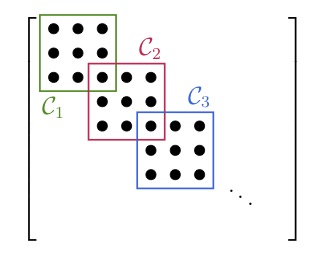
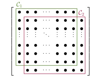
In the left figure we have the ideal case that all the blocks overlap in just one entry. A full decomposition would leave us with a large number of small blocks. The sparsity pattern in the right figure has two large blocks overlapping almost entirely. In this case it would be disadvantageous to decompose the blocks. Instead, we would do the initial decomposition, realize the large overlap, and then merge the two blocks back together. For sparsity patterns that arise from real applications the case is not always as clear and we have to use more sophisticated strategies to decide which blocks to merge.
COSMO currently provides three different strategies that can be selected by the user:
COSMO.NoMerge — Type
NoMerge <: AbstractMergeStrategyA strategy that does not merge cliques.
COSMO.ParentChildMerge — Type
ParentChildMerge(t_fill = 8, t_size = 8) <: AbstractTreeBasedMergeThe merge strategy suggested in Sun and Andersen - Decomposition in conic optimization with partially separable structure (2014). The initial clique tree is traversed in topological order and a clique $\mathcal{C}_\ell$ is greedily merged to its parent clique $\mathcal{C}_{par(\ell)}$ if at least one of the two conditions are met
- $(| \mathcal{C}_{par(\ell)}| -| \eta_\ell|) (|\mathcal{C}_\ell| - |\eta_\ell|) \leq t_{\text{fill}}$ (fill-in condition)
- $\max \left\{ |\nu_{\ell}|, |\nu_{par(\ell)}| \right\} \leq t_{\text{size}}$ (supernode size condition)
COSMO.CliqueGraphMerge — Type
CliqueGraphMerge(edge_weight::AbstractEdgeWeight = ComplexityWeight()) <: AbstractGraphBasedMergeThe (default) merge strategy based on the reduced clique graph $\mathcal{G}(\mathcal{B}, \xi)$, for a set of cliques $\mathcal{B} = \{ \mathcal{C}_1, \dots, \mathcal{C}_p\}$ where the edge set $\xi$ is obtained by taking the edges of the union of clique trees.
Moreover, given an edge weighting function $e(\mathcal{C}_i,\mathcal{C}_j) = w_{ij}$, we compute a weight for each edge that quantifies the computational savings of merging the two cliques. After the initial weights are computed, we merge cliques in a loop:
while clique graph contains positive weights:
- select two permissible cliques with the highest weight $w_{ij}$
- merge cliques $\rightarrow$ update clique graph
- recompute weights for updated clique graph
Custom edge weighting functions can be used by defining your own CustomEdgeWeight <: AbstractEdgeWeight and a corresponding edge_metric method. By default, the ComplexityWeight <: AbstractEdgeWeight is used which computes the weight based on the cardinalities of the cliques: $e(\mathcal{C}_i,\mathcal{C}_j) = |\mathcal{C}_i|^3 + |\mathcal{C}_j|^3 - |\mathcal{C}_i \cup \mathcal{C}_j|^3$.
See also: Garstka, Cannon, Goulart - A clique graph based merging strategy for decomposable SDPs (2019)
In our example problem we have two cliques $\mathcal{C}_3 = \{ 3,6,7,8\}$ and $\mathcal{C}_5 = \{6,7,8,9 \}$ that overlap in three entries. Let's solve the problem again and choose the default clique merging strategy merge_strategy = COSMO.CliqueGraphMerge:
model = JuMP.Model(with_optimizer(COSMO.Optimizer, decompose = true, merge_strategy = COSMO.CliqueGraphMerge));
@variable(model, x[1:2]);
@objective(model, Min, c' * x )
@constraint(model, Symmetric(B - A1  .* x[1] - A2 .* x[2] )  in JuMP.PSDCone());

JuMP.optimize!(model)
------------------------------------------------------------------
COSMO v0.5.0 - A Quadratic Objective Conic Solver
Michael Garstka
University of Oxford, 2017 - 2019
------------------------------------------------------------------
Problem: x ∈ R^{7},
constraints: A ∈ R^{30x7} (58 nnz),
matrix size to factor: 37x37 (153 nnz)
Sets: PsdConeTriangle of dim: 15
PsdConeTriangle of dim: 6
PsdConeTriangle of dim: 6
PsdConeTriangle of dim: 3
Decomp: Num of original PSD cones: 1
Num decomposable PSD cones: 1
Num PSD cones after decomposition: 4
Merge Strategy: CliqueGraphMerge
Settings: ϵ_abs = 1.0e-04, ϵ_rel = 1.0e-04,
ϵ_prim_inf = 1.0e-06, ϵ_dual_inf = 1.0e-04,
ρ = 0.1, σ = 1.0e-6, α = 1.6,
max_iter = 2500,
scaling iter = 10 (on),
check termination every 40 iter,
check infeasibility every 40 iter,
KKT system solver: QDLDL
Setup Time: 0.26ms
Iter: Objective: Primal Res: Dual Res: Rho:
40 -1.4134e+00 1.7924e-05 1.0416e-04 1.0000e-01
------------------------------------------------------------------
>>> Results
Status: Solved
Iterations: 40
Optimal objective: -1.4134
Runtime: 0.003s (2.68ms)Unsurprisingly, we can see in the output that COSMO solved a problem with four PSD constraints. One of them is of dimension 15, i.e. a $5\times 5$ block, which correspond to the merged clique $\mathcal{C_3} \cup \mathcal{C}_5 = \{3,6,7,8,9 \}$.
Completing the dual variable
After a decomposed problem is solved, we can recover the solution to the original problem by assembling the matrix variable $S$ from its subblocks $S_\ell$:
\[S = \displaystyle \sum_{\ell = 1}^p T_\ell^\top S_\ell T_\ell,\]
Following Agler's Theorem, $S$ will be a positive semidefinite matrix. However, this is not true for the corresponding dual variable matrix $Y$. The dual variable returned after solving the decomposed problem will be in the space of PSD completable matrices $Y \in \mathbb{S}_+^n(E,?)$. This means that the entries in $Y$ corresponding to the blocks $S_\ell$ (black dots) have been chosen correctly. The numerical values for all the other entries (corresponding to the zeros in $S$ and denoted with a red dot) have to be chosen in the right way to make $Y$ positive semidefinite.
For more information about PSD matrix completion and the completion algorithm used in COSMO take a look at Vandenberghe and Andersen - Chordal Graphs and Semidefinite Optimization (Ch.10). To configure COSMO to complete the dual variable after solving the problem you have to set the complete_dual option:
model = JuMP.Model(with_optimizer(COSMO.Optimizer, complete_dual = true));Example Code
The code used for this example can be found in /examples/chordal_decomposition.jl.