The source files for all examples can be found in /examples.
Support Vector Machine
We are showing how to solve a support vector machine problem with COSMO (and JuMP).
Generating the Dataset
We want to classify the points in this example dataset with $m = 100$ samples and $n = 2$ features:
using Distributions: MvNormal
using Plots, LinearAlgebra, SparseArrays, Random, Test
# Generate dataset
rng = Random.MersenneTwister(123);
num_samples = 100;
Xpos = rand(rng, MvNormal([1.5, 1.5], 1.25), div(num_samples, 2))';
Xneg = rand(rng, MvNormal([-1.5, -1.5], 1.25), div(num_samples, 2))';
ypos = ones(div(num_samples, 2));
yneg = -ones(div(num_samples, 2));# Plot dataset
plot(Xpos[:, 1], Xpos[:, 2], color = :red, st=:scatter, markershape = :rect, label = "positive", xlabel = "x1", ylabel = "x2")
plot!(Xneg[:, 1], Xneg[:, 2], color = :blue, st=:scatter, markershape = :circle, label = "negative")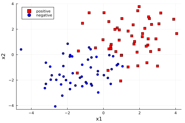
with samples $(x_1, x_2, \ldots, x_m) \in \mathbb{R}^2$ and labels $y_i \in \{-1,1\}$.
Solving SVM as a QP
We want to compute the weights $w$ and bias term $b$ of the (soft-margin) SVM classifier:
\[\begin{array}{ll} \text{minimize} & \|w\|^2 + \lambda \sum_{i=1}^m \text{max}(0, 1 - y_i(w^\top x_i - b)), \end{array}\]
where $\lambda$ is a hyperparameter. This problem can be solved as a quadratic program. We can rewrite above problem into an optimisation problem in primal form by introducing the auxiliary slack variables $t_i$:
\[t_i = \text{max}(0, 1 - y_i(w^T x_i - b)), \quad t_i \geq 0.\]
This allows us to write the problems in standard QP format:
\[\begin{array}{ll} \text{minimize} & \|w\|^2 + \lambda \sum_{i=1}^m t_i\\ \text{subject to} & y_i (w^\top x_i - b) \geq 1 - t_i, \quad \text{for } i = 1,\ldots, m\\ & t_i \geq 0, \quad \text{for } i = 1,\ldots, m. \end{array}\]
Next, we will remove the bias term $b$ by adding an initial feature $x_0 = -1$ to each sample (now: $n = 3$):
X = [-ones(num_samples) [Xpos; Xneg]];
y = [ypos; yneg];
m, n = size(X)
(100, 3)Modelling in JuMP
We can model this problem using JuMP and then hand it to COSMO:
using JuMP, COSMOλ = 1.0; # hyperparameter
model = JuMP.Model(optimizer_with_attributes(COSMO.Optimizer, "verbose" => true));
@variable(model, w[1:n]);
@variable(model, t[1:m] >= 0.);
@objective(model, Min, w' * w + λ * ones(m)' * t);
@constraint(model, diagm(0 => y) * X * w .+ t .- 1 .>= 0);
status = JuMP.optimize!(model)------------------------------------------------------------------
COSMO v0.8.11 - A Quadratic Objective Conic Solver
Michael Garstka
University of Oxford, 2017 - 2022
------------------------------------------------------------------
Problem: x ∈ R^{103},
constraints: A ∈ R^{200x103} (500 nnz),
matrix size to factor: 303x303,
Floating-point precision: Float64
Sets: Nonnegatives of dim: 200
Settings: ϵ_abs = 1.0e-05, ϵ_rel = 1.0e-05,
ϵ_prim_inf = 1.0e-04, ϵ_dual_inf = 1.0e-04,
ρ = 0.1, σ = 1e-06, α = 1.6,
max_iter = 5000,
scaling iter = 10 (on),
check termination every 25 iter,
check infeasibility every 40 iter,
KKT system solver: QDLDL
Acc: Anderson Type2{QRDecomp},
Memory size = 15, RestartedMemory,
Safeguarded: true, tol: 2.0
Setup Time: 0.86ms
Iter: Objective: Primal Res: Dual Res: Rho:
1 -1.2386e+03 1.8621e+01 7.9772e+00 1.0000e-01
25 2.0745e+01 1.9518e-01 2.2851e-01 1.0000e-01
50 2.1369e+01 7.2162e-02 4.2689e-03 1.0000e-01
75 2.1467e+01 4.3595e-02 4.6488e-02 1.0000e-01
100 2.1572e+01 2.8674e-02 1.4458e-03 1.0000e-01
125 2.1608e+01 2.5533e-02 1.1443e-02 1.0000e-01
150 2.1637e+01 3.2745e-02 3.7370e-03 1.0000e-01
175 2.1640e+01 8.4182e-03 8.8939e-04 1.0000e-01
200 2.1639e+01 8.2338e-03 1.5876e-05 1.0000e-01
225 2.1655e+01 3.5882e-03 1.4714e-01 5.7968e+00
250 2.1660e+01 4.8392e-03 5.5964e-02 4.5721e-01
275 2.1660e+01 1.1386e-03 4.3094e-03 4.5721e-01
300 2.1659e+01 4.7153e-04 3.3939e-03 4.5721e-01
325 2.1659e+01 5.2653e-04 2.8383e-05 4.5721e-01
350 2.1659e+01 5.2672e-04 1.0771e-05 4.5721e-01
375 2.1659e+01 5.2702e-04 6.3165e-05 1.0406e+01
400 2.1659e+01 5.2690e-04 4.1489e-05 1.0406e+01
425 2.1660e+01 4.8125e-05 8.0658e-03 1.0406e+01
450 2.1660e+01 2.8002e-04 4.1772e-03 5.9577e-01
475 2.1660e+01 1.6661e-04 6.8381e-04 5.9577e-01
500 2.1660e+01 1.6727e-04 9.1359e-05 7.8180e-02
525 2.1660e+01 1.8989e-06 2.0554e-06 7.8180e-02
------------------------------------------------------------------
>>> Results
Status: Solved
Iterations: 549 (incl. 24 safeguarding iter)
Optimal objective: 21.66
Runtime: 0.021s (20.9ms)The optimal weights $w = [w_0, w_1, w_2]^\top$ (where $w_0 = b$) are:
w_opt = JuMP.value.(w)3-element Vector{Float64}:
-0.12492307858082635
0.9045142793404424
0.780407893799139Plotting the hyperplane
The separating hyperplane is defined by $w^\top x - b = 0$. To plot the hyperplane, we calculate $x_2$ over a range of $x_1$ values:
\[x_2 = (-w_1 x_1 - w_0) / w_2, \text{ where } w_0 = b.\]
x1 = -4:0.1:4;
x2 = (-w_opt[2] * x1  .- w_opt[1]) / w_opt[3]
plot!(x1, x2, label = "SVM separator", legend = :topleft)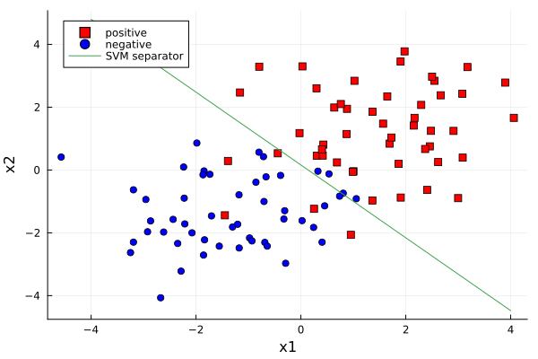
Modelling with COSMO
The problem can also be solved by transforming it directly into COSMO's problem format. Define COSMO`s $x$-variable to be $x=[w, t]^\top$ and choose $P$, $q$, accordingly:
P = blockdiag(spdiagm(0 => ones(n)), spzeros(m, m));
q = [zeros(n); 0.5 * λ * ones(m)];
Next we transform the first constraint $y_i (w^\top x_i - b) \geq 1 - t_i, \quad \text{for } i = 1,\ldots, m$ into COSMO's constraint format: $Ax + b \in \mathcal{K}$.
A1 = [(spdiagm(0 => y) * X) spdiagm(0 => ones(m))];
b1 = -ones(m);
cs1 = COSMO.Constraint(A1, b1, COSMO.Nonnegatives);
It remains to specify the constraint $t_i \geq 0, \quad \text{for } i = 1,\ldots, m$:
A2 = spdiagm(0 => ones(m));
b2 = zeros(m);
cs2 = COSMO.Constraint(A2, b2, COSMO.Nonnegatives, m+n, n+1:m+n);
Create, assemble and solve the COSMO.Model:
model2 = COSMO.Model();
assemble!(model2, P, q, [cs1; cs2]);
result2 = COSMO.optimize!(model2);
w_opt2 = result2.x[1:3];
@test norm(w_opt2 - w_opt, Inf) < 1e-3
Test PassedThis page was generated using Literate.jl.